Using Hugging Face on Quest

This tutorial will guide you through the steps of using a model from Hugging Face on Quest. It will walk through a Python script which includes accessing the model, tokenizing the data, fine-tuning the model, and running calculations in a python script using the fine-tuned model. It will also go over how to submit this as a batch job on Quest.

Hugging Face is an open-source platform which is a central hub for AI development and research. Using the Hugging Face API and the transformers library, you can load, train, and fine-tune models on Quest.

The sections below demonstrate how to determine the location where you will store your models, how to create a virtual environment with the required software to run your workflow, an example fine-tuning Python script, and an example submission script to run your job in batch on Quest.

This article assumes that you are already familiar with python, Quest, virtual environments, and have some knowledge on LLM implementation. If you are not familiar with these topics yet, please refer to the Quest User Guide, Python on Quest, and Virtual Environments on Quest pages.

Storing Hugging Face Models

In order to work with the models, you will first need to pull the model you want to work with to Quest. You will pull the model onto Quest as a part of your workflow, which we will explain further in the example Python code. where you want to store your model hashes should be defined prior to running your workflow.

When you pull models from Hugging Face in your workflow, the model hash will be stored, by default, in your home directory /home/<netid>/

For some bigger models, you may want to consider storing the model hashes somewhere else than in your home directory, since you only have 80GiB of storage in your home directory. To change the location where the model hashes are stored, run the following command:

echo "export HF_HOME=/scratch/<netID>/path/to/HF/.cache/huggingface/" >> $HOME/.bashrc

Instead of saving the models in scratch space, you can also make this location point to a directory in your /projects/pXXXXX folder. The key differences between scratch space and your projects space are:

• Your scratch space has 5TB of storage, whereas your projects directory has either 1 or 2TB of storage

• Data stored in your scratch space that has a “last modified” date that surpasses 30 days will automatically be deleted, whereas data stored in your projects directory will not be automatically deleted.

Based on the size of your model and how long you would like to keep it stored on Quest, you can make the decision whether to store it in your scratch space or in your projects directory.

Warning

Since Hugging Face is a repository for models to which anyone can contribute, be aware of models that do not come from a verified source. Malicious versions of models have been found. Malicious code has particularly been found in files in pickle and other serialization formats.

Creating a Virtual Environment including Hugging Face

If you want to use Hugging Face models in your batch jobs on Quest, you will need to create a virtual environment that contains the Transformers and Unsloth packages, as well as all the other packages your Python script requires. Transformers provides you with everything you need for inference or training with models, while Unsloth helps with efficiency of the jobs. To read more about virtual environments, please see our article on mamba or conda virtual environments.

First, load the mamba module on Quest:

$ module load mamba/24.3.0

Next, create a virtual environment with Python, Transformers, Unsloth, and any other packages you need. The --prefix argument creates the virtual environment in a specified location, rather than in the default location (/home/<net_id>/.conda/envs/). Since Transformers has PyTorch as a dependency, we also add that package to the environment.

$ mamba create --prefix=/projects/p12345/envs/huggingface-env -c conda-forge python=3.12

$ mamba activate /projects/p12345/envs/huggingface-env 

$ mamba install pytorch-cuda=12.1 pytorch nvidia/label/cuda-12.1.0::cuda-toolkit xformers -c pytorch -c nvidia -c xformers

$ pip install unsloth # Unsloth needs to be installed with pip for functionality purposes

Example Workflow

One way to work with LLMs on Quest is to use the models that are available through Hugging Face. The workflow outlined below uses a python script called fine_tuning.py. The full workflow and all files necessary to run this workflow can be found on our GitHub page . It might be helpful to reference this full script while reading through this tutorial, as we will break down parts of the script below.

fine_tuning.py is a sample script which uses the Hugging Face package to load in a model and fine tune it on the IMDB dataset for sentiment analysis that is provided by the Python package datasets. This dataset is often used as a benchmark for binary sentiment analysis, as it contains 50,000 movie reviews that are highly polarized that are labeled as either positive or negative. In our code, the model’s objective is to categorize the movies in the dataset correctly as either positive or negative.

The first thing you have to do in the fine_tuning.py script is set up all the packages you need to import in order for your script to run.

### Imports ###

# HuggingFace libraries
from transformers import AutoTokenizer, AutoModelForSequenceClassification, TrainingArguments, Trainer, pipeline
from datasets import load_dataset, concatenate_datasets
import evaluate

# Machine learning
from sklearn.metrics import confusion_matrix, ConfusionMatrixDisplay, classification_report, roc_curve, auc, precision_recall_curve, average_precision_score

# Misc
import numpy as np
from collections import Counter
import matplotlib.pyplot as plt

After loading in the necessary packages, we will load in the IMDB data from datasets. We will only select a small percentage of the whole data. Note that the dataset has all the 0 (negative) labels first, so instead of taking the first N samples, we take a random sample from each of the labels. Taking a random sample means that we randomly choose a subset of data from each label. Luckily, datasets loading is “lazy” so it doesn’t load everything into memory right away, so we can do the following:

### Load Data ###

dataset = load_dataset("imdb", split="train")

neg_dataset = dataset.filter(lambda x: x['label'] == 0).select(range(250))
pos_dataset = dataset.filter(lambda x: x['label'] == 1).select(range(250))

dataset = concatenate_datasets([neg_dataset, pos_dataset]).shuffle(seed=42)

print(Counter(dataset["label"]))

Now that we have the data loaded in, we will create a model by first tokenizing the data, which is the process of converting “sub-words” to numbers, as the model can only deal with numbers and not with text. Once the data has been tokenized, we will create the fine-tuned classification model:

### Create Model and Train ###

# Model Name
model_name = "distilbert-base-uncased"

# Tokenizing
tokenizer = AutoTokenizer.from_pretrained(model_name)
def preprocess(text_sample):
    return tokenizer(text_sample["text"], truncation=True, padding="max_length", max_length=128)

tokenized_dataset = dataset.map(preprocess, batched=True)

# Create Fine-Tuned Classification Model
model = AutoModelForSequenceClassification.from_pretrained(model_name, num_labels=2)

The model above that is listed as the variable pulls an already established Hugging Face model (BERT) and gets a classification pipeline for it. This is the base model on which the trainer will work to fine-tune the model. Fine-tuning will alter the model slightly so that it is more specific to our data.

Before we start training the model, we have to define the accuracy metric. When you want to know if your model is doing well, you need a way to assess what “doing well” means. In this case, we look for an accuracy that looks for “Did you get the label (0/negative or 1/positive) right?” If it’s a positive review, and the model classifies it as such, your model gets a “score” of +1. If it classifies it as negative when it is positive, it will get 0. When this is done over the whole datasets, you will get a percentage of times that the model was correct, which is the overall accuracy.

# Define accuracy metric
accuracy = evaluate.load("accuracy")

def compute_metrics(pred):
    preds = np.argmax(pred.predictions, axis=1)
    return accuracy.compute(predictions=preds, references=pred.label_ids)

Now, we create our trainer:

# Training setup
training_args = TrainingArguments(
    output_dir="./test_fine_tuning",
    per_device_train_batch_size=4,
    num_train_epochs=1,
    logging_steps=10,
    save_steps=1000,
    push_to_hub=False,  # disable pushing to HF
    report_to="none",  # disable logging to wandb (weights and biases) and other places - otherwise it asks for API key
)

trainer = Trainer(
    model=model,
    args=training_args,
    train_dataset=tokenized_dataset,
    tokenizer=tokenizer,
    compute_metrics=compute_metrics
)

From the training arguments, the most important ones are the per_device_train_batch_size and num_train_epochs variables.

per_device_train_batch_size specifies how many samples you provide to the neural network at each iteration. If you give it a lot of data points at once, it might be too much for the network to process and could run out of memory. If you only give it one sample, it will learn in a very noisy way, which is also not desired. For the purpose of running this workflow on Quest, using a batch size of 4 is a good amount. However, the more powerful your computer is, the bigger your batch size can be.

num_train_epochs defines how many times you go over your entire dataset. Once you have gone over all of the batches of data points, you will have completed one epoch. For example, with the settings above and using 100 data points, you will have 25 batches (four data points per iteration) and one epoch.

Once we have set the training arguments, we start training the model:

trainer.train()

After you train the model, we need to evaluate the results and how well the model did. For evaluation, we need to get the testing dataset and tokenize it. We do this by loading a test split. Remember that the data is not balanced. so you load and filter by label 0 or 1:

### Evaluate ###
test_dataset = load_dataset("imdb", split="test")

# Filter 250 negative and 250 positive samples
test_neg = test_dataset.filter(lambda x: x['label'] == 0).select(range(250))
test_pos = test_dataset.filter(lambda x: x['label'] == 1).select(range(250))

test_dataset = concatenate_datasets([test_neg, test_pos]).shuffle(seed=42)

# Tokenize
tokenized_test = test_dataset.map(preprocess, batched=True)

Now we can evaluate:

trainer.evaluate(tokenized_test)

We now have our fine-tuned model. Let’s predict the label for some example tests. The first step is to create a classification pipeline with our model:

### Predict ###

classif_pipeline = pipeline("text-classification", model=model, tokenizer=tokenizer)
classif_pipeline("Wow, this is the worst movie I've seen in my entire life")
classif_pipeline("Wow, this is the best movie I've seen in my entire life")
classif_pipeline("Wow, I don't know how to feel about it")

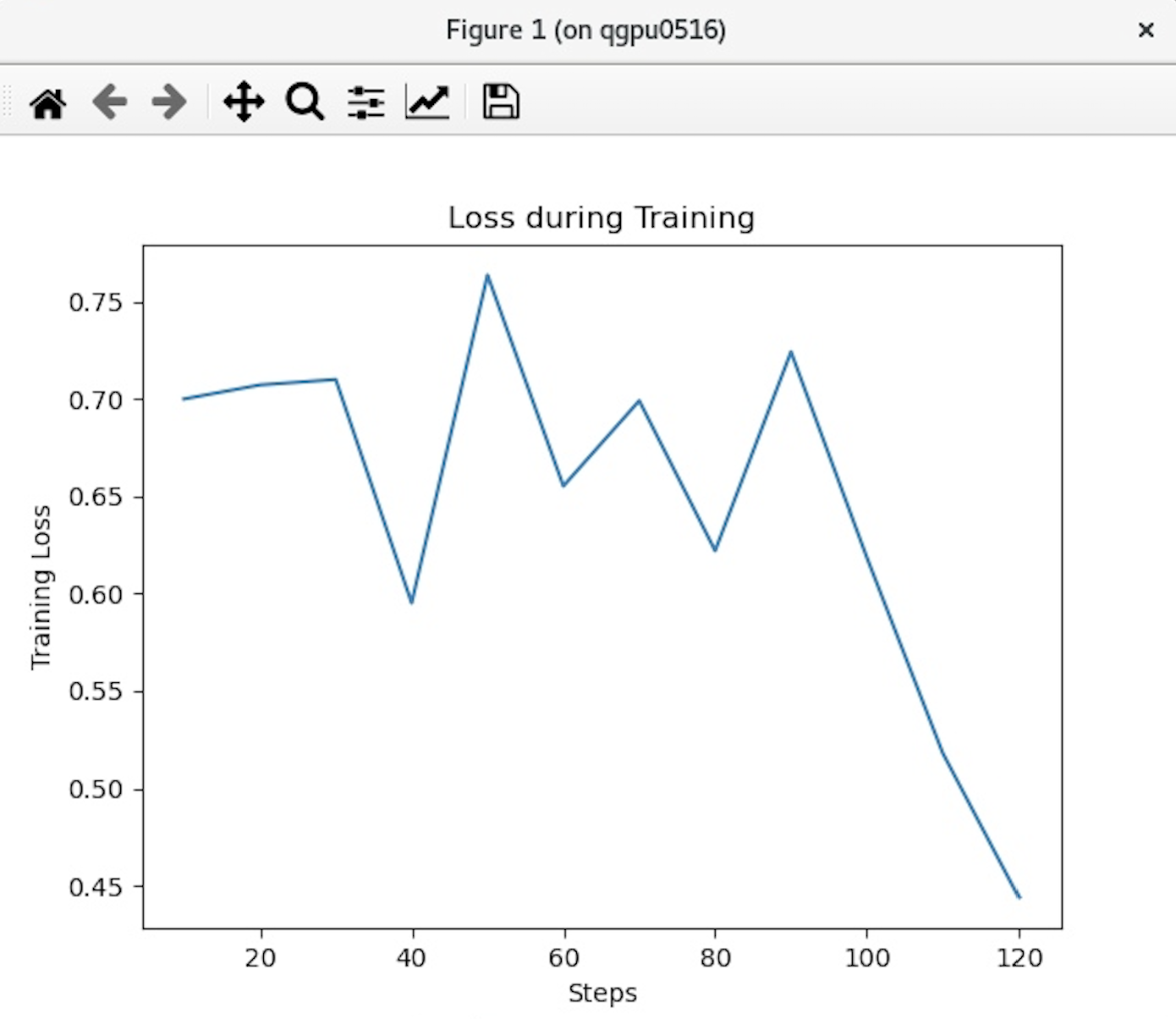
Based on this classification, we can make some visualizations. First, we will visualize the error evolution during training:

### Visualizations ###
# Training evolution
logs = trainer.state.log_history

loss = [entry['loss'] for entry in logs if 'loss' in entry]
steps = [entry['step'] for entry in logs if 'loss' in entry]

plt.plot(steps, loss)
plt.xlabel("Steps")
plt.ylabel("Training Loss")
plt.title("Loss during Training")
plt.show()

In the plot, you can see that the loss is going down, which means the model is getting more accurate. Loss is the function with which algorithms are trained. It tries to find the weights of the neural network that mathematically minimizes the loss.

Next, we will plot performance metrics using a confusion matrix:

# Performance Metrics
preds = trainer.predict(tokenized_test)
y_true = preds.label_ids
y_pred = preds.predictions.argmax(axis=1)

disp = ConfusionMatrixDisplay.from_predictions(y_true,y_pred, display_labels=["Negative", "Positive"], cmap = 'Greys')

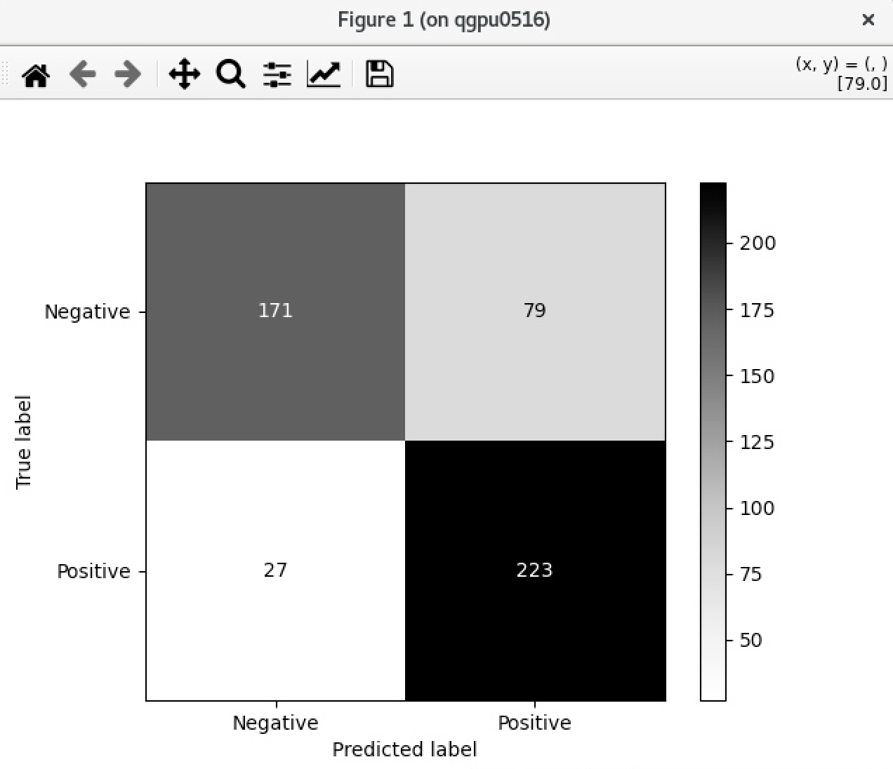
The confusion matrix shows how accurate the model was in categorizing the movies as positive or negative. If the movies were categorized as negative in the dataset, how many times did the model accurately predict that the movie was negative? Looking at the matrix above, you can see that:

• There were 171 samples that were negative, and the model predicted as negative.

• There were 27 samples that were negative, but the model predicted as positive.

• There were 79 samples that were positive, but the model predicted as negative.

• There were 223 samples that were positive, and the model predicted as positive.

To assess whether your model performed well, you want to see high numbers in the left top and bottom right elements, as these are your accurate predictions. Additionally, you want to see low numbers in the left bottom and top right elements, as these are your errors.

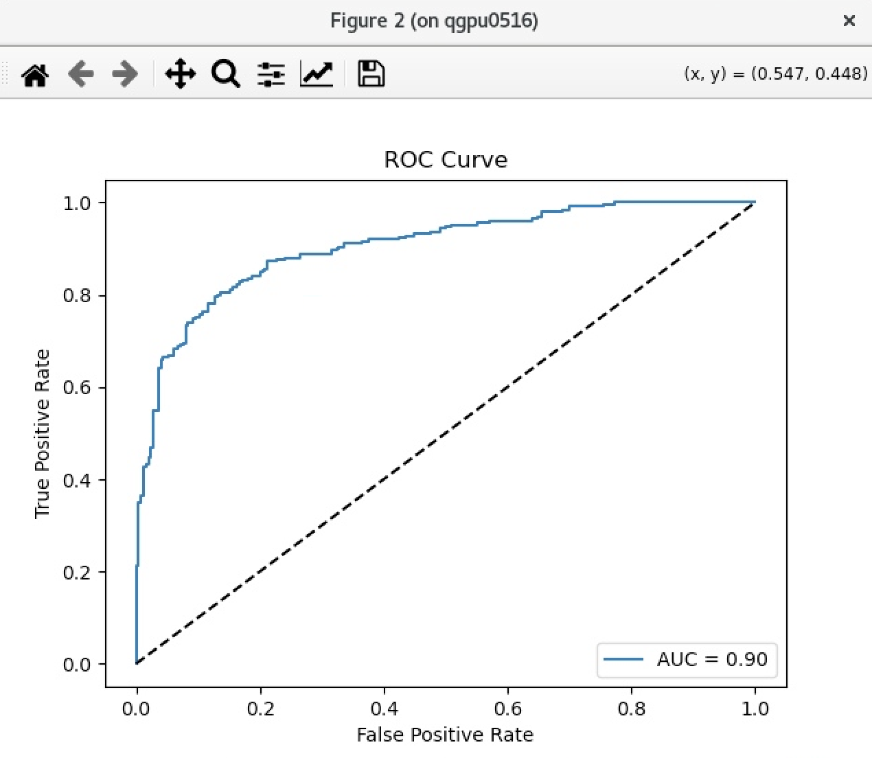
Next, we will make an ROC (Receiver Operating Characteristic) curve. In the ROC curve, each point represents a threshold, and at each threshold the model makes certain errors, meaning it incorrectly classifies a movie as positive or negative. The ROC curve shows us the false positive (a sample was classified as positive by the model when it wasn’t) rate for each threshold. This creates a curve. The greater the AUC (Are Under Curve), the better our model works. In other words, you will want to see a curve that bends as much possible to the top left.

# ROC Curve
y_scores = preds.predictions[:, 1]  # score for class 1 (positive)
fpr, tpr, thresholds = roc_curve(y_true, y_scores)
roc_auc = auc(fpr, tpr)

plt.figure()
plt.plot(fpr, tpr, label=f"AUC = {roc_auc:.2f}")
plt.plot([0, 1], [0, 1], "k--")
plt.xlabel("False Positive Rate")
plt.ylabel("True Positive Rate")
plt.title("ROC Curve")
plt.legend(loc="lower right")
plt.show()

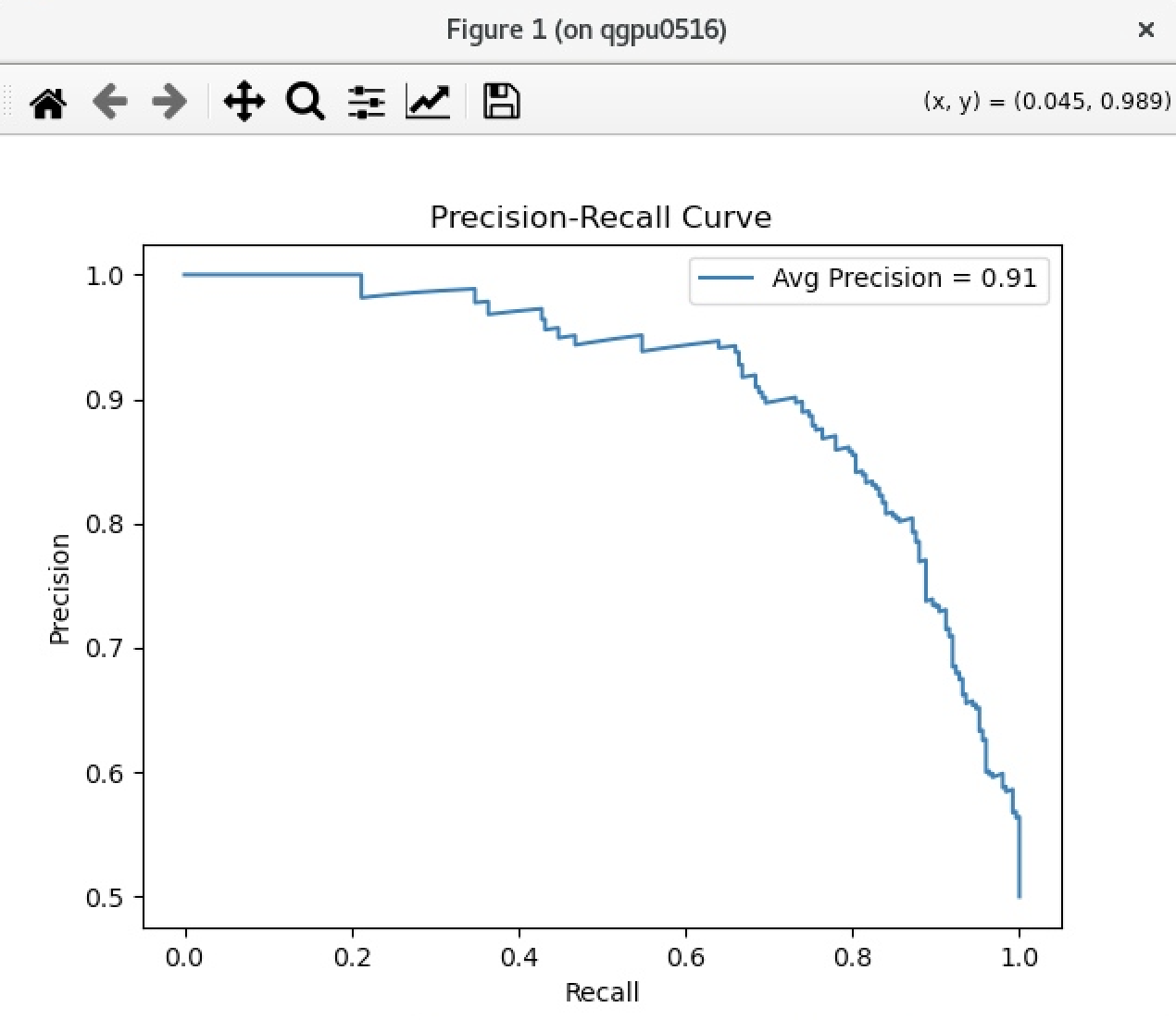
Lastly, we create a Precision-Recall Curve. This curve is similar to the ROC Curve, but instead of looking at the false/true positive rate, it looks at the precision versus the recall. Precision = Among all the samples that the model guessed were positive, how many were actually positive. Recall = Among all the samples that were positive, how many did the model correctly guess as positive.

# Precision recall curve
precision, recall, thresholds = precision_recall_curve(y_true, y_scores)
avg_precision = average_precision_score(y_true, y_scores)

plt.plot(recall, precision, label=f"Avg Precision = {avg_precision:.2f}")
plt.xlabel("Recall")
plt.ylabel("Precision")
plt.title("Precision-Recall Curve")
plt.legend()
plt.show()

You can use both ROC and Precision-Recall curves for similar outcomes when you have an equal amount of data for both categories you are working with. However, if you have more data for one category than the other, you should use the Precision-Recall curve instead of the ROC curve. For example, if your model poorly predicts positively rated movies, but overall performs well, the ROC curve would not show this. However, the Precision-Recall curve would show you this detail about your model.

Running your LLM script on Quest as a Batch Job

To run the above script, fine_tuning.py, as a batch job on Quest, use the submission script submit-fine-tuning.sh.

First, here is an example of the SBATCH flags you can use to submit this job. It is likely that you don’t have to change anything besides your allocation and email. However, if you make changes to downsample size, model type, or other Hugging Face-specific variables, the time and amount of GPU cards may need to be altered.

#!/bin/bash
#SBATCH --account=pXXXX  ## YOUR ACCOUNT pXXXX or bXXXX
#SBATCH --partition=gengpu  ### PARTITION (buyin, short, normal, etc)
#SBATCH --nodes=1 ## how many computers do you need
#SBATCH --ntasks-per-node=4 ## how many cpus or processors do you need on each computer
#SBATCH --job-name=HuggingFace-batch-job ## When you run squeue -u <NETID> this is how you can identify the job
#SBATCH --time=3:30:00 ## how long does this need to run 
#SBATCH --mem=40GB ## how much RAM do you need per node (this effects your FairShare score so be careful to not ask for more than you need))
#SBATCH --gres=gpu:1 ## type of GPU requested, and number of GPU cards to run on
#SBATCH --output=output-%j.out ## standard out goes to this file
#SBATCH --error=error-%j.err ## standard error goes to this file
#SBATCH --mail-type=ALL ## you can receive e-mail alerts from SLURM when your job begins and when your job finishes (completed, failed, etc)
#SBATCH --mail-user=email@northwestern.edu ## your email, non-Northwestern email addresses may not be supported

If you have any additional questions on how to set up a job or about the SBATCH flags, please refer to this page on the Slurm job scheduler, or specifically on Slurm configuration settings.

Next, we will need to unload any previously loaded modules and load in our module to use our virtual environment. If you have any other modules to load in, you would do that here as well:

module purge
module load mamba/24.3.0

The last steps of the submission script activate the virtual environment and run the python script you want to run. These are really the only lines you will need to edit in this entire script (besides any SBATCH flags or module versions if your code requires it). Make sure that you change the path to your virtual environment as well as the name of your python script if you are using a different script.

# activate virtual environment
eval "$('/hpc/software/mamba/24.3.0/bin/conda' 'shell.bash' 'hook' 2> /dev/null)"
source "/hpc/software/mamba/24.3.0/etc/profile.d/mamba.sh"
mamba activate /projects/p12345/envs/huggingface-env # Make sure to change the path of this environment to point to where your virtual environment is located.

#Run the python script
python -u /path/to/python/script/fine_tuning.py

If you have any questions regarding this tutorial, please feel free to submit a ticket by emailing quest-help@northwestern.edu .