Scaling Studies on Quest

Overview

A scaling study measures how application performance changes as computational resources increase. Specifically, it helps you identify how long your code takes to run when you use different numbers of cores or nodes because performance usually does not scale linearly with the number of cores or nodes. The goal is to identify an efficient number of cores to use for your job so you can avoid requesting and using resources that will not meaningfully reduce the runtime of your application.

Consider running a scaling study when the work to conduct a study is likely to have a net benefit for your workflow. You might benefit from a scaling study when:

• Your code can flexibly scale to use varying numbers of cores and/or nodes.

• You will need to run the same code many times, either over time or across different datasets or inputs.

• The code takes a significant amount of time to run.

Scaling studies help balance time-to-solution (how fast a job completes) with resource efficiency (how many cores are used), and are essential for:

• Requesting the right resources for your workflow

• Avoiding over-allocation of cores or nodes

• Understanding the performance bottlenecks in parallel applications

• Producing defensible performance results for publications

On shared systems like Quest, larger jobs often wait longer in the scheduler queue because they require more resources (cores or nodes) to become available at the same time. Scaling studies help you understand how much time you’re likely to gain by splitting your job across more cores.

This page introduces core scaling concepts, explains limits to parallel performance, and outlines how to perform a scaling study on Quest. By the end of this guide, you will be able to design, run, and interpret a scaling study to identify an efficient core count for your application on Quest.

Before You Begin

To follow this guide, you should:

• Have access to Quest and be able to submit jobs

• Have a working application or workflow you want to run at scale

• Be able to run your application on a single core or small number of cores

Running Example: A Simple Scaling Study

To make these concepts concrete, we will use a simple example throughout this guide.

Suppose you have a Python program that estimates π using a Monte Carlo method. The program:

• Generates random points

• Checks whether they fall inside a circle

• Repeats this many times to improve accuracy

This workload can be parallelized by splitting the work across multiple CPU cores, where each core processes a subset of the total number of samples.

We will use this example to illustrate:

• How speedup and efficiency are calculated

• Why scaling eventually slows down

• How to interpret scaling results on Quest

A full implementation of this example is described later in this guide, but we introduce it here to ground the concepts that follow.

What Do We Mean by Speedup and Efficiency?

To interpret scaling results, we use quantitative metrics that describe how performance changes as the number of cores increases. Two closely related concepts, speedup and parallel efficiency, are used to measure how much faster a parallel run is compared to a baseline, and how effectively additional cores are being utilized.

These metrics help answer practical questions such as whether adding more cores meaningfully reduces runtime, and where increasing cores begins to yield diminishing returns. Together, speedup and efficiency form the basis for analyzing scaling behavior.

Speedup

The most basic metric in a scaling study is speedup, which is defined as:

Speedup = Serial Runtime / Parallel Runtime

This measures how much faster your application runs on multiple cores compared to a single core.

In an ideal world, doubling the number of cores would halve the runtime, leading to linear speedup:

• 2 cores → 2× speedup

• 4 cores → 4× speedup

• N cores → N× speedup

In practice, ideal (1:1) scaling is rare beyond very small core counts.

In our π example, speedup measures how much faster the Monte Carlo simulation runs as we distribute the samples across more cores.

Parallel Efficiency

Parallel efficiency is often used alongside speedup:

Efficiency = Speedup / Number of Cores = (T₁ / Tₙ) / N

Where:

• T₁ = baseline runtime

• Tₙ = runtime on N cores

For the π example, efficiency tells us whether adding more worker processes actually leads to productive work, or whether overhead begins to dominate. Efficiency close to 1 (or 100%) indicates good scaling, while rapidly decreasing efficiency signals diminishing returns as resource counts increase.

Why Real Applications Don’t Scale Perfectly

While ideal linear scaling is a useful reference point, real scientific and engineering applications almost never achieve it beyond small core counts. As parallel resources increase, a variety of algorithmic, runtime, and system-level factors introduce overhead that limits performance gains.

Understanding why scaling breaks down is as important as measuring speedup. These limitations help explain where adding more cores stops being beneficial and provide insight into whether performance bottlenecks arise from the application design, the parallelization strategy, or hardware constraints.

Amdahl’s Law

Amdahl’s Law formalizes a fundamental constraint on parallel performance:

• Some fraction of your program is inherently serial

  • For example, initializing input data, reading from disk, writing output files, or combining results at the end of a computation are often performed by a single process and cannot be parallelized

• No amount of additional parallel resources can accelerate that serial portion

As core count increases, runtime eventually becomes dominated by the serial fraction, causing speedup to plateau. In the π example, tasks like initializing the random number generator or aggregating results at the end are performed serially and cannot be parallelized.

For scaling studies, the practical takeaway is simple:

At sufficiently large core counts, adding more resources will no longer reduce runtime in a meaningful way.

Common Sources of Scaling Overhead

Beyond serial code, several real-world effects reduce scaling efficiency:

• Communication, coordination, and synchronization overhead

• Memory and I/O effects

• Runtime and system noise

The sections below briefly describe each of these sources of overhead and explain how they can limit scalability as resource counts increase.

Communication, Coordination, and Synchronization Overhead

Parallel applications incur overhead when work is distributed across multiple processes and results must be coordinated or combined. This is true regardless of the programming model used (MPI, threading, task-based runtimes, or workflow engines).

Common sources of overhead include:

• Inter-process or inter-thread communication

  • Any exchange of data between parallel tasks, which can become significant when communication occurs between nodes

  • Examples include:

    • MPI point-to-point messages

    • Sending results through task queues or runtime systems

• Collective coordination

  • Points in a parallel program where multiple tasks must communicate or wait for each other before continuing

  • Examples include:

    • Barriers - where all tasks must reach the same point before any can proceed

    • Reductions - where values from all tasks are combined into a single result

    • Broadcasts - where the same data is sent from one task to all others

• Load imbalance

  • Uneven distribution of work or data across tasks

  • Faster tasks waiting for slower ones before progressing

As resource counts increase, these effects increasingly force parallel tasks to wait for one another, causing coordination overhead to grow faster than useful computation and limiting achievable scalability.

Memory and I/O Effects

As applications scale, performance can become limited by how quickly data can be accessed or written, rather than by raw compute capacity. Memory and I/O bottlenecks often emerge when many tasks compete for shared hardware resources. Examples include:

• Bandwidth limitations on shared memory systems

• File system contention when many ranks perform I/O simultaneously

Runtime and System Noise

Performance variability can also arise from factors outside of the application itself. On shared systems like Quest, runtime and system-level effects can introduce noise that becomes more visible at larger scales. For example:

• Scheduler placement effects (e.g., how processes are distributed across nodes or racks)

• Background system activity

• Variability in network performance

Types of Scaling Studies

There are multiple ways to evaluate how an application scales, depending on whether the problem size changes as resources increase. The two most common approaches are weak scaling and strong scaling.

To make the distinction concrete, we return to the running example introduced earlier: a Monte Carlo simulation that estimates π by generating random samples and checking whether they fall inside a circle.

Weak Scaling

In a weak scaling study, the problem size increases proportionally with the number of cores.

This asks: “If I make my problem bigger, can I keep my runtime constant?”

Example (π simulation):

• Suppose each core processes 2 million random samples

• on 1 core → 2 million data points

• on 8 cores → 16 million data points

• on 32 cores → 64 million data points

In this setup, each core always does the same amount of work. As you add cores, you increase the total number of samples being computed.

If the application scales well, the runtime should stay approximately the same as you add cores, because no individual core is doing more work than before.

Weak scaling tells you how well your application can handle larger problems. In the π example, it answers whether you can increase the number of samples (and therefore improve accuracy) without increasing runtime.

Common use cases:

• Increasing the resolution or fidelity of a simulation

• Processing growing datasets

• Expanding workloads as more resources become available

Strong Scaling

In a strong scaling study, the total problem size is held constant while the number of cores or nodes increases.

This asks: “If my problem stays fixed, how much faster can I finish it?”

Example (π simulation):

• Suppose you want to compute 64 million total samples

• On 1 core → one process handles all 64 million samples

• on 8 cores → each core processes 8 million samples

• on 32 cores → each core processes 2 million samples

As you add cores, the same total work is divided into smaller pieces.

If the application scales well, runtime should decrease as more cores are added, since the work is being completed in parallel.

Strong scaling tells you how effectively you can reduce time-to-solution for a fixed problem. In the π example, it measures how quickly you can finish generating the same number of samples.

Real-world use cases

• Reducing runtime for a fixed simulation or dataset

• Meeting deadlines for analyses or production workloads

• Determining the most efficient resource request on shared systems like Quest

Strong scaling studies are most appropriate when:

• The problem size is fixed by physical or scientific constraints

• Minimizing time-to-solution is the primary goal

The rest of this page focuses on strong scaling, as it is the most common and practical approach for Quest users and for determining efficient resource requests.

When Should You Do a Scaling Study?

Scaling studies require running the same workload multiple times with different resource configurations. Because this can be time-consuming, they are most useful when you expect to run a workflow repeatedly or at large scale.

You should consider performing a scaling study when:

• Your job will be run many times (e.g., parameter sweeps, production workflows)

• Your job is computationally expensive (hours to days of runtime)

• You are unsure how many cores or nodes to request

• You want to avoid long queue wait times from over-requesting resources

• You need defensible performance data (e.g., for publications or reports)

In contrast, a full scaling study may not be necessary for:

• One-off or exploratory jobs

• Very short jobs where runtime differences are negligible

• Workflows that are inherently serial or cannot effectively use multiple cores

Should You Use Your Full Workflow?

In most cases, you do not need to run a scaling study on your largest or most expensive production workload. Instead, the goal is to use a representative version of your problem that:

• Preserves the same computational structure

• Exercises the same performance bottlenecks

• Runs quickly enough to repeat multiple times

How to Scale Down a Problem

A good scaling-study workload should behave like your real application, just at smaller scale. Common strategies include:

• Reduce problem size

  • Fewer simulation elements (e.g., smaller grid, fewer particles)

  • Fewer data points or iterations

  • In the π example: reduce the total number of samples

• Reduce input data volume

  • Use a subset of your dataset

  • Process fewer files or shorter time ranges

• Preserve parallel structure

  • Keep the same number of tasks per core or similar workload decomposition

  • Ensure communication patterns remain similar (if applicable)

• Maintain realistic runtime

  • Each run should still take long enough (e.g., minutes rather than seconds) to expose meaningful performance differences

The key idea is: your scaled-down version should reflect the same performance behavior as your real workload, even if it is much smaller.

Be careful not to reduce the problem size so much that startup, communication, scheduling, or I/O overhead dominates the runtime. In general, larger problems tend to scale better because there is more useful work to distribute across cores.

For example, a Monte Carlo π calculation with only a small number of samples may stop scaling at low core counts because process-management overhead becomes a significant fraction of the runtime. The same application with billions of samples may continue scaling efficiently to many more cores.

A useful approach is to test a few problem sizes. If doubling the problem size significantly changes the shape of your scaling results or shifts the point where speedup begins to level off, the smaller problem is probably not representative of your production workload. Continue increasing the problem size until scaling behavior is relatively stable.

As a rule of thumb, the useful computation should dominate the runtime. If a run completes in only a few seconds, startup and scheduling overhead may have a disproportionate impact on the results. Scaling studies are often more reliable when each run takes at least several minutes.

Practical Guideline

A useful rule of thumb: A single run in your scaling study should take long enough to measure performance reliably but be short enough to repeat across many configurations.

Performing a Scaling Study on Quest

We now walk through a complete scaling study on Quest using the Monte Carlo π example introduced earlier. This example illustrates how to apply the concepts of strong scaling, speedup, and efficiency in practice.

In this study, the goal is to answer a practical question: How many cores should I request to run this workload efficiently on Quest?

Problem Setup

The application estimates π by generating random points and checking whether they fall inside a circle. The total amount of work is fixed, making this a strong scaling study.

The workload consists of:

• 8,192 independent tasks

• 2,000,000 samples per task

• ~16 billion total samples

Each task is independent, so the workload is embarrassingly parallel and parallelized using Python’s multiprocessing module.

The scaling study runs the same code multiple times using different numbers of cores to compare how long the full task takes to complete. Each run of the code provides a data point to understand the scaling behavior.

A complete, runnable version of this scaling study—including job scripts and analysis code—is available in our repository of example jobs on GitHub .

Step 1: Choose a Baseline Configuration

Once you have defined a representative workload (as described above), start by selecting a baseline configuration for your scaling study.

In this example:

• A single-core run is used as the baseline

• All 16 billion samples are processed by one process/CPU

This provides the reference runtime (T₁) used to compute speedup and efficiency.

More generally, a good baseline should:

• Use the same workload and configuration as all other runs

• Be simple and reliable (often 1 core or a small core count)

• Serve as a consistent point of comparison across all scaling results

This baseline answers: How long does the entire workload take without parallelism?

Step 2: Design a Consistent Set of Runs that Scales

To ensure meaningful comparisons, all runs use:

• The same Python script and input parameters

• The same software environment

• The same node type and memory allocation

• The same total workload (16 billion samples)

Only one parameter should vary across runs:

• Number of CPU cores

Changing the number of cores changes the amount of work each core does. For our example, as the number of cores increases, each core processes fewer samples.

The study sweeps across core counts:

1, 2, 4, 6, 8, 10, 16, 20, 32, 40, 64, 80, 128

Because our example uses Python multiprocessing (a shared-memory model), we restrict the study to a single node to isolate scaling effects such as task scheduling and memory contention. This avoids introducing additional overhead from communication between nodes. Therefore we run the study using the resources of a single node, increasing core counts from 1 to 128. You might choose different core counts for your study.

To do this yourself, write a script to submit these jobs using different core counts (see the example ). To get accurate results, you may want to run each configuration (core count) multiple times to account for the variability on Quest from things you cannot control.

Note

While this example is limited to a single node, the approach generalizes to other types of applications:

• Shared-memory applications (e.g., multiprocessing, OpenMP) are typically limited to a single node

• Distributed-memory applications (e.g., MPI) can scale across multiple nodes

For multi-node applications, scaling studies often vary the number of nodes in a consistent way (e.g., 1 node, 2 nodes, 4 nodes), ideally using full nodes at each step to ensure consistent hardware usage.

Step 3: Verify That Your Code Is Actually Using Multiple Cores

While a parallel job is running, or after the jobs finish, check to make sure that your code is actually using multiple cores.

The example application uses multiprocessing.Pool, launching one worker process per core. In the context of this example, verifying parallelism means confirming:

• Each core is processing a portion of the Monte Carlo samples

• Work is actually distributed rather than running serially

To do this:

• Use top to verify active processes while your job is running

  1. Identify the compute node your job is running on (from your job output or tools such as squeue <netid> or sacct <netid>).

  2. Connect to that node:

     ssh <qnodeXXX>
     

  3. Run:

     top -u <netid>
     

  4. Find your job’s processes

  5. Verify correct behavior:

     • You should see multiple processes (typically one per core requested).

     • Each process should show non-zero CPU usage (often near 100% for CPU-bound jobs).

     • If only one core is active, the simulation is effectively running serially, and any scaling results will be misleading or invalid.

• Use seff <jobid> to check overall job efficiency after your job has finished

  1. After your job finishes, run:

     seff <jobid>
     

  2. Look for key metrics in the output:

     • CPU Efficiency

       • In general, ~70% or higher is a good target

       • Higher values (~80–90%) are typical for well-parallelized, compute-bound workloads

       • Example: If you request 16 cores for a 10-minute job, the maximum possible CPU time is:

         • 16 cores × 10 minutes = 160 CPU-minutes

         • If seff reports 144 CPU-minutes used, that corresponds to 90% efficiency (144/160)

         • If it reports 80 CPU-minutes, that corresponds to 50% efficiency (80/160)

     • CPU Utilized

       • Total CPU time consumed across all cores (e.g., core-hours or core-seconds)

       • Should increase as you use more cores and/or run longer jobs

  3. Interpret results:

     • High CPU efficiency ≥ 70% → generally indicates good resource utilization

     • CPU efficiency well below 70% → possible underutilization, I/O bottlenecks, or misconfiguration

Step 4: Record Runtime and Compute Metrics

For each run:

• Record total runtime from scheduler output

  • You can find the runtime by using the seff command

  • seff <jobid>
    

    and record the reported “Job Wall-clock time”

• Compute:

  • Speedup = T₁ / Tₙ

  • Parallel efficiency = Speedup / N

In this example:

df['speedup'] = baseline_runtime / df['elapsed']
df['efficiency'] = df['speedup'] / df['ncpus']

Note that this efficiency is computed from runtime measurements and reflects parallel scaling behavior, while the CPU efficiency reported by seff measures how fully allocated CPU resources were utilized during a job.

These metrics answer:

• How much faster the π computation becomes

• Whether added cores are being used effectively

Results and Interpretation

Speedup

The speedup curve shows how much faster the computation becomes as cores are added.

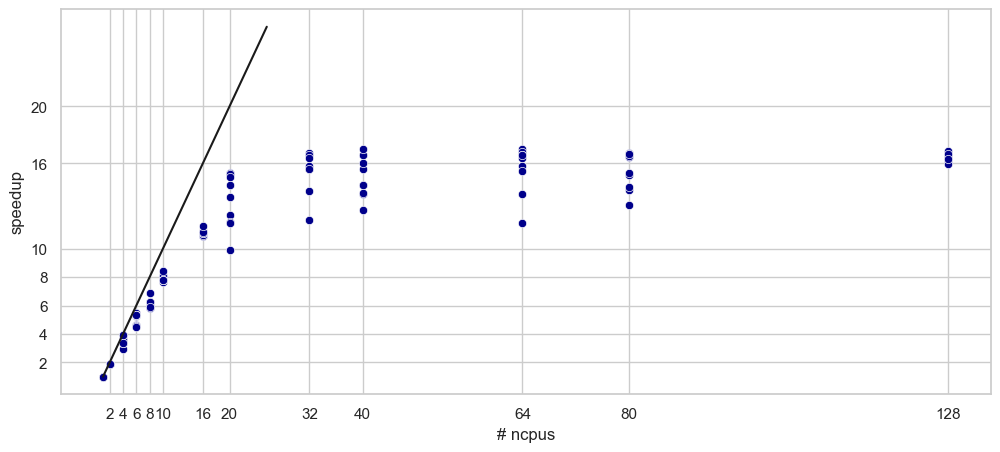
Speedup versus core count for a strong scaling study of the Monte Carlo π application. Experimental measurements (blue markers) are compared against the theoretical linear speedup limit (black line).

Observed behavior:

• Near-linear scaling at small core counts (1–8 cores)

• Deviation from linear scaling starting in the range of 16–32 cores

• Plateau around a 16x speedup for 32–40 cores

Even though the workload is embarrassingly parallel, the speedup eventually stops improving.

Parallel Efficiency

The efficiency plot shows how quickly the overall use of resources becomes less efficient as more resources are used.

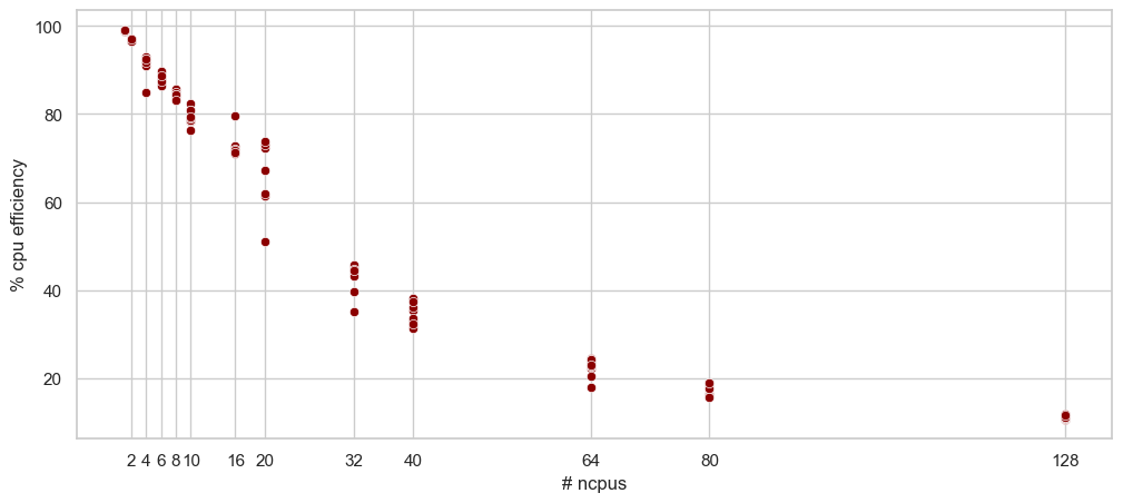
Parallel efficiency versus core count for the Monte Carlo π application. Efficiency is computed as speedup divided by core count and illustrates the decreasing effectiveness of additional cores at larger scales.

Observed behavior

• High efficiency (~90–100%) at small core counts

• Steady decline in efficiency as cores increase

• At large scale:

  • 64 cores → ~20–25% efficiency

  • 128 cores → ~10–12% efficiency

This indicates many cores are underutilized at large scale.

Interpretation

To understand why speedup levels off in this example, we look at factors that introduce overhead as the number of processes increases. These effects limit how effectively additional cores can be used.

In the π example, scaling limitations arise from:

• Task scheduling overhead in multiprocessing: Managing and distributing many small tasks to worker processes introduces overhead that grows with the number of processes.

• Result aggregation (a serial component): Partial results from each worker must be collected and combined, which cannot be fully parallelized.

• Memory bandwidth contention on a shared node: As more processes run simultaneously, they compete for access to memory, limiting performance gains.

• Load imbalance between worker processes: Some tasks may finish earlier than others, causing idle time while waiting for all processes to complete.

Practical Takeaway

For this workload, an efficient configuration is ~16–32 cores per node.

This range provides:

• Strong speedup gains

• Reasonable efficiency

• Minimal wasted resources

Beyond this point:

• Runtime improves only marginally

• Efficiency drops sharply

• Additional cores provide little benefit

Summary

This example demonstrates a typical strong scaling pattern:

• Good scaling at low core counts

• Slowing gains at moderate scale

• Clear plateau at higher core counts

Even for a highly parallel workload like Monte Carlo π, more cores do not always lead to faster results.

Scaling studies like this help identify the point where additional resources stop being useful, allowing you to make efficient and effective resource requests on Quest.